Research Study
Introduction
This study analyzes climate change, specifically CO2 emissions around the world. This is accomplished by comparing the variables of population and GDP (Gross Domestic Product) in different countries and correlating them with CO2 emissions. The purpose of this is to see the relationships between each variable individually, as well as how they affect the problem combined.
Climate change is a change in climate patterns, which is highly attributed to Carbon Dioxide emissions being released into the atmosphere by the burning of fossil fuels. This climate change is evident by a rise in global temperature, devastating weather changes, and CO2 filling the atmosphere.
This study hypothesizes that the variables of population and GDP will have an effect on countries CO2 emission rates; the effect of emission rates can go up or down depending on these variables and how they cohesively make an impact. The study will also assess the individual impact that each variable has on CO2 emission rates.
The purpose of this study is to have a better understanding of how regression analysis is used to compare variables as well as see how future predictions of CO2 emissions may be impacted by a rise in population combined with GDP. Previous studies have looked into population as a variable in CO2 emissions but not at how multiple variables can cohesively show results in per country CO2 emissions. This is helpful because the comparison of the variables and their relationships could help predict future CO2 emissions as countries show an increase or decrease in residents as well as economic level.
Objectives
- Complete a regression analysis of GDP (Gross Domestic product) and population in different countries.
- See the relationships between GDP and population within different countries.
- Use those relationships to foresee future CO2 emissions per county by its increase or decrease in population and economic level.
|
Figures
Figure 1. Equation shows how to solve for the B2 variable, (the slope of GDP) which is calculated by taking the sum of each varying X.
Figure 2. Table of data collected from each of the ten countries. 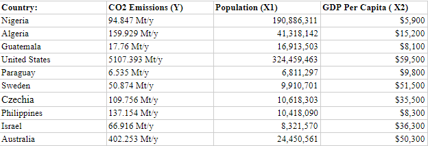
Figure 3. Regression plane of the data collected, showing the predicted rise in CO2 emissions relatively, and in a planar fashion. 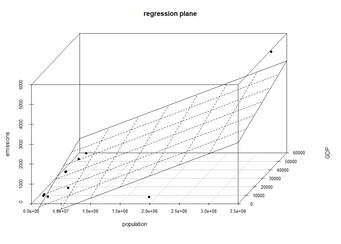
|
Methods In order to study the effects on this problem, subjects must be selected for best fit. In this case, that means choosing what countries will be analyzed and referenced. This study focused on ten countries which were selected using a random country generator. Even though this was a randomized process, there was one qualification in that there must be at least one country from each continent (not including Antarctica). This way there would not be an uneven or swayed sample. The countries studied were as follows: Mayotte (Africa), Algeria (Africa), Guatemala (North America), United States of America (North America), Paraguay (South America) , Sweden (Europe), Czechoslovakia (Europe), Philippines (Asia), Israel (Asia), and Australia (Oceania). Two variables were gathered for each country: Population as of 2017 and Gross Domestic Product (GDP). GDP is a quantitative measure of countries total economic activity. This is calculated by [consumption +government expenditures +investment +exports -imports = GDP]. Originally, the idea of economic level was one of the variables focused on. However it can be difficult to classify countries based on first, second, and third world characteristics, since they are so broad. As an alternative, GDP has physical numbers than can be associated with each country, making the data analysis clearer. The results of this study have been organized and defined using a regression analysis of emissions data from the selected countries. Regression analysis is a statistical method used to look at relationships between different variables. In regression analysis, there are typically one to three variables that are being compared using different statistical techniques. The main way this is accomplished is through using t-tests and f-tests to do a comparison. T-tests are used primarily to look at the probability between two sets of data. In other words, to evaluate a variable’s individual effect on the problem. F-tests are used to determine the relationship and effect the variables have on the problem simultaneously. For this study, there was a global f-test that was used to show how all observed variables interact and how their combined CO2 emissions fluctuate as a result. Then a t-test was performed on each of the independent variables (population and GDP) in order to see their individual contribution to CO2 emissions. In order to see the relationships between these variables clearly, five of the countries regressions were performed by hand in order to better understand the process. This specific equation, Figure 1, was used to calculate the B2, which gives the GDP slope, (Figure 2). Similarly, B1 is the slope of the population variable. The primary researcher consulted a research statistics consultant to make sure the equations and calculations were accurate, they originally acquired these equations from an online source. In addition, all ten regression analysis of the countries were done on a program called R-studio. R-studio is a programming software designed to compare data for analysis and research. The regression f-test was also performed by hand to see how the variables actually interact with each other. When done on r-studio all of the calculations are done automatically and not shown completely; by doing a regression by hand it is clear where the B1 and B2 and other statistics come from. All of the data was then compiled into a plane graph to visualize the f-test results and the final results of how population and GDP impact a rise or loss in CO2 emissions. |
Results
From each of the ten countries studied, data was gathered as presented in Figure 2. CO2 emissions are measured in Metric tons per year (Mt/y). GDP is measured per capita, which is the country's Gross Domestic Product divided by the total population in regards to how it relates to each citizen.
Based on the results of the global f-test, R2=.83. This indicates that 83 percent of variants in the model are explained by two variables (Population, GDP). R2 is determined by the equation R2=SSmodel/SStotal; SSmodel= Σ(Ŷ-ỹ)2 SStotal= Σ(y-ỹ). Also calculated was B1 (population relationship) and B2 (GDP relationship). B1 and B2 are calculated by the action shown in Figure 1. B1 was equal to 1.116323*10-5. As population increases it can be calculated through this regression that for every one million people, CO2 emissions rise by 11.16323 Mt/y. This data is gathered from the calculation, [B1*1,000,000]. B2 was equal to .02570598. Similarly, it was calculated by [B2*500], indicating that every $500 more GDP per capita increases CO2 emissions by 12.853 Mt/y.
Another aspect of this study is the p value for this model. P value is used to show the likelihood of each variables outcome happening by coincidence. Typically if the p value is less than 5 percent, it shows that the relationships are genuine and significant contributors to CO2 emissions. Overall p value was .001953 or 0.19 percent. The variable population’s individual p value was .00227 or 0.227 percent. GDP individual p value was equal to .07372 or 7.3 percent.
This means that based on calculated p values, all data is statistically significant in the results.The p value for GDP was 7.3 percent which is over the 5 percent general cut off. This means that basing CO2 emissions purely on GDP however would probably not give accurate results for future predictions. However, since the overall p value is .19 percent (which is lower than the population's .277), it can be concluded that population and GDP combined give the most significant predictor of emissions.
As stated above, there were three variables being measured. CO2 emissions, population, and GDP. Therefore, for a graph to represent this data accurately it can not be a two dimensional X and Y axis graph. The third dimension of this study and the slope is demonstrated in a three dimensional plane.
Using r-studio, a 3-dimensional plane plotted the data from the countries with population on the x-axis, emissions on the y-axis, and GDP on the X2 or z-axis. This graph depicts the predicted current trend in CO2 emissions; it shows the relationship between the variables. (Figure 3). The graph also shows that as population and GDP of a country increases, the emissions will increase in a predicted planar fashion.
Conclusions
The results of the f-test coincided with the original hypothesis, that GDP and population have a combined significant effect on CO2 emissions. This is supported by the 83 percent variance that was calculated, which is used to represent the amount of impact the two variables combined have on CO2 emissions. In other words GDP and population help to explain 83% of the variation in CO2 emissions.
The outliers in this data set are the United States, which had a higher population and GDP per capita than mathematically predicted by its emissions. Another outlier is Nigeria, which has a high population but low GDP, and which produces lower emission rates than expected. In this study, these outliers were included in order to represent the varying sides of countries and how additional variables come into play in certain countries’ CO2 emissions. If there were multiple countries included whose emissions exceeded beyond others think the slope would have been skewed heavily. Although the United States has much higher emissions for their population, it was offset by Nigeria’s low emissions for their population.
Through the results of the study of ten different countries’ carbon dioxide emissions, not only can see the significance of these variables in rise in CO2 emissions, but also the impact Gross Domestic Product can have when predicting future global emissions.
However, there are limited outcomes of research like this. Results can not be represented in a generalized sense as they occur. Additionally when any regression analysis is performed even through software like R-studio, the data can get very messy quickly would likely be impossible.
Future Research
Previously, studies have focused on the region, regulation, and population individually with respect to CO2 emissions. This study focused on population and economic level and how they interact together, since the effect of GDP combined with population have not been an avenue of research prior to now. The results of this study show the relationship that these variables have and how much impact they have on predicting and current CO2 emissions, as observed by the slope of the plane of the regression graph. A lot of the big discussions occurring now are based around prevention or stopping emissions in the future. When looking at the current situation, a predicted number such as this can be used to help inform countries and policy makers when determining where focus towards emissions control needs to go and how to prevent the continual increase in atmospheric CO2 globally. Lowered CO2 emissions can have the benefits of saving money, saving the planet, and providing a better future for generations to come.
Previously, studies have focused on the region, regulation, and population individually with respect to CO2 emissions. This study focused on population and economic level and how they interact together, since the effect of GDP combined with population have not been an avenue of research prior to now. The results of this study show the relationship that these variables have and how much impact they have on predicting and current CO2 emissions, as observed by the slope of the plane of the regression graph. A lot of the big discussions occurring now are based around prevention or stopping emissions in the future. When looking at the current situation, a predicted number such as this can be used to help inform countries and policy makers when determining where focus towards emissions control needs to go and how to prevent the continual increase in atmospheric CO2 globally. Lowered CO2 emissions can have the benefits of saving money, saving the planet, and providing a better future for generations to come.
